Debugging a Logic Circuit in IDP-Z3

In my previous blog post, I showed how we can solve a puzzle in the IDP-Z3 reasoning engine. It was inspired by a post by Hillel Wayne, who modelled the puzzle in Prolog. He starts the article by stating how, for his book, he prefers showing off logic programming through practical examples instead of small puzzles, which I quite agree with. Here's the good news: in this post, I'll show you how the puzzle was actually a practical problem in disguise, and how it can be generalised to, e.g., the debugging of logic circuits¹. :-)

Abstracting the puzzle

A brief re-cap of the puzzle: we are given test answers and corresponding results for three students, and have to use this information to deduce the score of a fourth student. Crucially, we are not given the correct answers -- this is the puzzle, of course! We can abstract it as follows:

Given a description of a system's internal workings, together with a series of input-output observations, deduce information on an unknown aspect of the system.

It is easy to see how this applies to the Layton puzzle:

• System: a test containing of 10 A-B questions, each worth 10 points if correct.
• Observations: students' answers and their scores.
• Goal: deduce the correct answers, and calculate the fourth student's score.

This abstract version can be applied to many more problem domains. For instance, it could be used for machine diagnosis: consider a broken machine for which we can describe the expected inner workings, and for which we have a series of observations. Or, as we'll show in the next section, we can also apply it to the debugging of logic circuits.

Logic Circuit

Imagine the following logic circuit, consisting of five gates (A-E):

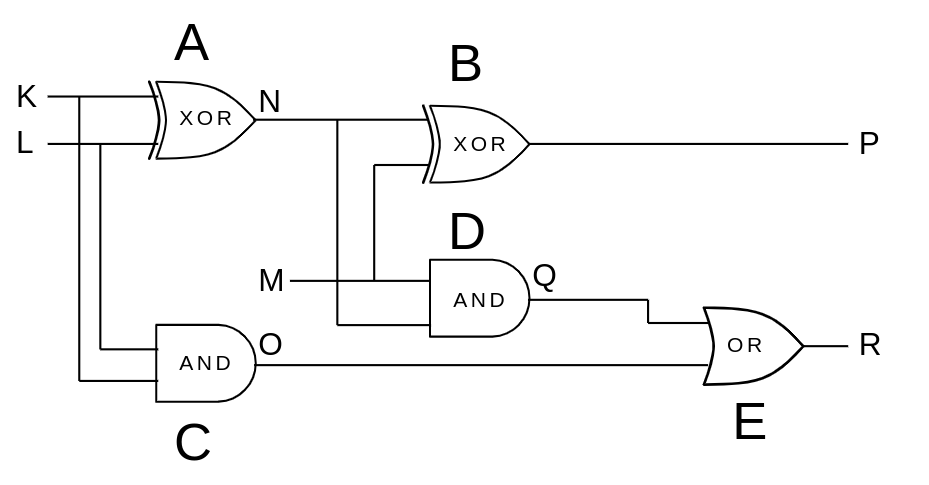
Somehow, it does not work as its supposed to, and our goal is to help diagnose the issue. Due to its design, however, it's not possible to read the pin-outs of the internal wires. Instead, we are given a set of three tests, consisting of the values of the input wires {K, L, M} and corresponding output values for output wires {P, R}. Does this look familiar, yet? :-)

Using the observations shown below, we should try to find a diagnosis for our system. As there will obviously be many possibilities, let's assume Occam's razor and try to look for the diagnosis in which the least amount of gates would need to be broken.

Test	K	L	M	P	R
1	1	0	0	1	1
2	0	1	0	1	1
3	0	0	1	1	0

Solving using IDP-Z3

We'll now show a solution in the IDP-Z3 reasoning engine. Like in the Layton puzzle, we'll start by creating a vocabulary block to declare the required symbols. Keep in mind that, in a normal setting, you'd build up such a vocabulary piece by piece, together with the structure and theory blocks. Unfortunately, though explaining this design proces is didactically interesting, it will make this post at least five times longer. If you'd like a short primer on IDP-Z3's FO(·) language, see the previous post or my Sudoku solver in IDP-Z3.

Vocabulary

To start our vocabulary, we need a way to represent the gates and the wires. In this case, we can straightforwardly use types and unary predicates as follows:

type Gate := {A, B, C, D, E}
// Following three predicates are used to denote the Gate's type
xor: Gate -> Bool
and: Gate -> Bool
or: Gate -> Bool

type Wire := {K, L, M, N, O, P, Q, R}
// Denote the in-/output wires of our circuit
input_wire: Wire -> Bool
output_wire: Wire -> Bool

We also introduce functions as a way to refer to each gate's in- and output wires.

output: Gate -> Wire
first_input: Gate -> Wire
second_input: Gate -> Wire

Next, we need a way to express the information related to the observations. For this purpose, we introduce a type Test together with some binary predicates to denote the value of wires during each test.

type Test := {1..3}

// Value of each wire during each test.
on: Wire * Test -> Bool

// Value of the observed input and output wires for each test.
input_on: Wire * Test -> Bool
input_off: Wire * Test -> Bool
observed_on: Wire * Test -> Bool
observed_off: Wire * Test -> Bool

Lastly, we introduce a unary predicate to denote broken gates, and an Integer constant to count the number of broken gates present in a circuit.

broken: Gate -> Bool
nb_broken: -> Int

With our vocabulary done, we can now move on to the structure.

Structure

In our structure, we can define the values for symbols that we already know. For instance, the circuit in the diagram shown above looks as follows:

xor := { A, B }.
and := { C, D }.
or  := { E }.

output 	    := { A -> N, B -> P, C -> O, D -> Q, E -> R }.
first_input  := { A -> K, B -> N, C -> L, D -> M, E -> Q }.
second_input := { A -> L, B -> M, C -> K, D -> N, E -> O }.

input_wire  := { K, L, M }.
output_wire := { P, R }.

To finish our structure, we now also interpret the symbols with the observed values of each test.

input_on := {(K, 1), (L, 2), (M, 3)}.
input_off := {(L, 1), (M, 1), (K, 2), (M, 2), (K, 3), (L, 3)}.
observed_on  := {(P, 1), (R, 1), (P, 2), (R, 2), (P, 3)}.
observed_off := {(R, 3)}.

Theory

Finally, we move on to the real meat and bones of our solution: the theory! Here, we express the formulas that actually describe the behavior of our system. In total, we want to express three pieces of knowledge.

1. What the behavior of a correct gate looks like.
2. How the observed input/output wires relate to the actual wires.
3. How to count the number of broken gates.

For brevity's sake, I'll only show the formula describing the AND gate:

!g in Gate, t in Test:
    and(g) & ~broken(g) 
    => (on(first_input(g), t)  & on(second_input(g), t) 
        <=> on(output(g), t)).

In words: "For every AND gate that's not broken must hold that there is an AND relationship between its input and output wires for each test".

Next, we express the relation between "input_on/off", "observed_on/off", and "on" as follows:

// Set the values of the inputwires for each test.
!w in Wire, t in Test: input_on(w, t) => on(w, t).
!w in Wire, t in Test: input_off(w, t) => ~on(w, t).

// Set the observed output values for each test.
!w in Wire, t in Test: observed_on(w, t)  =>  on(w, t).
!w in Wire, t in Test: observed_off(w, t) => ~on(w, t).

Lastly, we define how to count the number of broken gates using a cardinality operator:

// Count the number of gates that are broken.
nb_broken() = #{x in Gate: broken(x)}.

And we're done! We can now have IDP-Z3 look for the smallest set of broken gates, giving us the following solutions:

 Model 1
==========
on := {(K, 1), (L, 2), (M, 3), (N, 1), (N, 2), (O, 1), (O, 2), (P, 1), (P, 2), (P, 3), (R, 1), (R, 2)}.
broken := {C}.
nb_broken := 1.


Model 2
==========
on := {(K, 1), (L, 2), (M, 3), (N, 1), (N, 2), (P, 1), (P, 2), (P, 3), (Q, 1), (Q, 2), (R, 1), (R, 2)}.
broken := {D}.
nb_broken := 1.


Model 3
==========
on := {(K, 1), (L, 2), (M, 3), (N, 1), (N, 2), (P, 1), (P, 2), (P, 3), (R, 1), (R, 2)}.
broken := {E}.
nb_broken := 1.

Relying on Occam's razor, there's three gates that could be the culprit: C, D, or E. This concludes our formal model. :-)

I hope this post convincingly showed that the prof. Layton puzzle is actually a real life problem in disguise. I'm quite certain there are many similar problems out there, waiting to be solved using a knowledge-based approach.

If you are interested to see the knowledge base for yourself, you can check it out in our online environment. Eager to learn more about IDP-Z3? Visit our website or our interactive tutorial site.

^{[1] Thanks to colleagues Marc Denecker and Joost Vennekens for helping me realise this.}